Causal Cognition: Tutorial 1
Nicolas Navarre, Jan 30 2025
Utils
import numpy as np
from pgmpy.models import BayesianNetwork
from pgmpy.factors.discrete import TabularCPD
from pgmpy.inference import VariableElimination
import pgmpy as pgm

def make_collider(U_a=0.5,U_b = 0.5, theta_ac = .95, theta_bc = 0.95,conj=False):
    collider = BayesianNetwork(
        [('A','C'),
         ('B','C')
        ]
    )

    # These are inferres from the conditional probabiities given
    # would be good to generalize to more variables and create larger cpds
    if not conj:
        p_c_ab = theta_ac + theta_bc - theta_ac * theta_bc
    else:
        p_c_ab = theta_ac * theta_bc
    p_c_b_na = (theta_bc - p_c_ab * U_a ) / (1-U_a) if U_a != 1 else 0
    p_c_a_nb = (theta_ac - p_c_ab * U_b ) / (1-U_b) if U_b != 1 else 0


    p_c = [0, p_c_b_na, p_c_a_nb, p_c_ab]
    if any([x<0 for x in p_c]):
        raise ValueError("Impossible model specifications!")
    p_nc = [1-x for x in p_c]

    collider_cpd = [p_nc,p_c]

    cpd_a = TabularCPD(variable='A', variable_card=2, values=[[1-U_a], [U_a]])
    cpd_b = TabularCPD(variable='B', variable_card=2, values=[[1-U_b], [U_b]])
    cpd_c = TabularCPD(variable='C', variable_card=2, values= collider_cpd, evidence=['A','B'], evidence_card=[2,2])

    collider.add_cpds(
        cpd_a,
        cpd_b,
        cpd_c,
    )
    return collider

def make_fork(U_a=0.7, p_B_cond_A = 0.8,p_C_cond_A= 0.2):
    fork = BayesianNetwork(
        [('A','B'),
         ('A','C')
        ]
    )
    cpd_a = TabularCPD(variable='A', variable_card=2, values=[[1-U_a], [U_a]])
    cpd_b = TabularCPD(variable='B', variable_card=2, values=[[1,1-p_B_cond_A], [0,p_B_cond_A]], evidence=['A'], evidence_card=[2])
    cpd_c = TabularCPD(variable='C', variable_card=2, values=[[1,1-p_C_cond_A], [0,p_C_cond_A]], evidence=['A'], evidence_card=[2])
    fork.add_cpds(cpd_a,
                  cpd_b,
                  cpd_c
                 )
    return fork

def make_chain(U_a=0.7, p_B_cond_A = 0.8,p_C_cond_B= 0.8):
    chain = BayesianNetwork(
        [('A','B'),
         ('B','C')
        ]
    )
    cpd_a = TabularCPD(variable='A', variable_card=2, values=[[1-U_a], [U_a]])
    cpd_b = TabularCPD(variable='B', variable_card=2, values=[[1,1-p_B_cond_A], [0,p_B_cond_A]], evidence=['A'], evidence_card=[2])
    cpd_c = TabularCPD(variable='C', variable_card=2, values=[[1,1-p_C_cond_B], [0,p_C_cond_B]], evidence=['B'], evidence_card=[2])
    chain.add_cpds(cpd_a,
                  cpd_b,
                  cpd_c
                 )
    return chain
Recap
Casual strength and structure
Some measures of causal power with two variables $C$ (cause) and $E$ (effect).
$\Delta P = P(E|C) - P(E|\neg C)$
Power-PC = $\frac{\Delta P}{1-P(E|\neg C)}$
From causal strength to causal structure
Consider different strucures:
$ E \rightarrow C$
$ E \leftarrow C$
$ E , C$ (independent)
Instead of Power$_C (E)$ find $P(C \rightarrow E$) amongst the different structures.
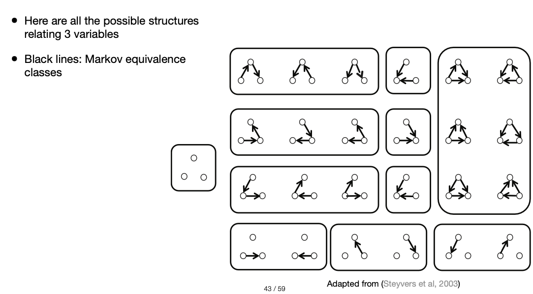
With more variables the strucrure inference becomes more complex:
Explaining away and Screening off
Screening off
This is a property of causal models where two variables are independent conditioned on another variable ($X \perp \!\!\! \perp Y | Z$)
Characteristic of chains:
$ X \rightarrow Z \rightarrow Y$
and forks:
$ X \leftarrow Z \rightarrow Y$
fork = make_fork()
fork.to_daft().render()
<Axes: >

fork_inference = VariableElimination(fork)
print('The joint probability distribution (every possible outcome):')
print(fork_inference.query(fork.nodes))
The joint probability distribution (every possible outcome):
+------+------+------+--------------+
| A    | B    | C    |   phi(A,B,C) |
+======+======+======+==============+
| A(0) | B(0) | C(0) |       0.3000 |
+------+------+------+--------------+
| A(0) | B(0) | C(1) |       0.0000 |
+------+------+------+--------------+
| A(0) | B(1) | C(0) |       0.0000 |
+------+------+------+--------------+
| A(0) | B(1) | C(1) |       0.0000 |
+------+------+------+--------------+
| A(1) | B(0) | C(0) |       0.1120 |
+------+------+------+--------------+
| A(1) | B(0) | C(1) |       0.0280 |
+------+------+------+--------------+
| A(1) | B(1) | C(0) |       0.4480 |
+------+------+------+--------------+
| A(1) | B(1) | C(1) |       0.1120 |
+------+------+------+--------------+
print('Probability of C knowing noting about the values of the system:')
print('P(C)')
print(fork_inference.query(['C']))
Probability of C knowing noting about the values of the system:
P(C)
+------+----------+
| C    |   phi(C) |
+======+==========+
| C(0) |   0.8600 |
+------+----------+
| C(1) |   0.1400 |
+------+----------+
print('Probability of C knowing its causal parent A happened:')
print('P(C|A=1)')
print(fork_inference.query(['C'],evidence={'A':1}))
Probability of C knowing its causal parent A happened:
P(C|A=1)
+------+----------+
| C    |   phi(C) |
+======+==========+
| C(0) |   0.8000 |
+------+----------+
| C(1) |   0.2000 |
+------+----------+
print('Probability of C knowing its causal parent A happened as well as sibling B happened:')
print('P(C|A=1,B=1)')
print(fork_inference.query(variables=['C'],evidence = {'A':1,'B':1}))
Probability of C knowing its causal parent A happened as well as sibling B happened:
P(C|A=1,B=1)
+------+----------+
| C    |   phi(C) |
+======+==========+
| C(0) |   0.8000 |
+------+----------+
| C(1) |   0.2000 |
+------+----------+
Notice that $P(C|A)=P(C|A,B)$. This is because $A$ screens off $C$ and $B$ in this structure!
Explaining away
This is a property of causal models, colliders in particular, where two unconditionally indepentent variables become dependent upon conditioning on another variable.
$X\rightarrow Z \leftarrow Y$
$X \perp \!\!\! \perp Y$ but $X \perp Y | Z$
Computational example
collider = make_collider(U_a=0.5,U_b=0.5)
collider.to_daft().render()
<Axes: >

collider_inference = VariableElimination(collider)
print('The joint probability distribution (every possible outcome):')
print(collider_inference.query(collider.nodes))
The joint probability distribution (every possible outcome):
+------+------+------+--------------+
| A    | C    | B    |   phi(A,C,B) |
+======+======+======+==============+
| A(0) | C(0) | B(0) |       0.2500 |
+------+------+------+--------------+
| A(0) | C(0) | B(1) |       0.0244 |
+------+------+------+--------------+
| A(0) | C(1) | B(0) |       0.0000 |
+------+------+------+--------------+
| A(0) | C(1) | B(1) |       0.2256 |
+------+------+------+--------------+
| A(1) | C(0) | B(0) |       0.0244 |
+------+------+------+--------------+
| A(1) | C(0) | B(1) |       0.0006 |
+------+------+------+--------------+
| A(1) | C(1) | B(0) |       0.2256 |
+------+------+------+--------------+
| A(1) | C(1) | B(1) |       0.2494 |
+------+------+------+--------------+
print('Probability of A knowing nothing about the values of the system:')
print('P(A)')
print(collider_inference.query(['A']))
Probability of A knowing nothing about the values of the system:
P(A)
+------+----------+
| A    |   phi(A) |
+======+==========+
| A(0) |   0.5000 |
+------+----------+
| A(1) |   0.5000 |
+------+----------+
print('Probability of A knowing its child C happened:')
print('P(A|C=1)')
print(collider_inference.query(['A'],evidence={'C':1}))
Probability of A knowing its child C happened:
P(A|C=1)
+------+----------+
| A    |   phi(A) |
+======+==========+
| A(0) |   0.3220 |
+------+----------+
| A(1) |   0.6780 |
+------+----------+
print('Probability of A knowing its child C happened and its co-parent B happened:')
print('P(A|C=1,B=1)')
print(collider_inference.query(['A'],evidence={'C':1,'B':1}))
Probability of A knowing its child C happened and its co-parent B happened:
P(A|C=1,B=1)
+------+----------+
| A    |   phi(A) |
+======+==========+
| A(0) |   0.4750 |
+------+----------+
| A(1) |   0.5250 |
+------+----------+
Note that $P(A=1|C=1)>P(A=1|C=1,B=1)$
This is known as explaining away
Bayes' Theorem
$$ P(H|D) = \frac{P(D|H)P(H)}{P(D)} $$
Cancer Mammogram
- 80% of mammograms detect breast cancer when it is there
- 9.6% of mammograms detect breast cancer when it’s not there
- 1% of women have breast cancer
$P(M=1|C=1) = 0.8$
$P(M=1|C=0) = 0.096$
$P(C=1) = 0.01$
$P(C=1|M=1)?$
$$P(C=1|M=1) = \frac{P(M=1|C=1)P(C=1)}{P(M=1)}$$
Now let's break down $P(M=1)$:
All possible ways in which you can have a positive mammogram:
- Having cancer (true positive)
- Not having cancer (false positive)
$$P(M=1) = P(M=1|C=0)P(C=0) + P(M=1|C=1)P(C=1)$$
# Given statistical data
tp = 0.8
fp = 0.096
p_cancer = 0.01

# Probability of a positive mamogram
p_M = fp*(1-p_cancer) + tp * p_cancer

# posterior probability of cancer
p_cancer_M = (tp * p_cancer)/p_M

print('P(C=1|M=1) =', f'{round(p_cancer_M*100,2)}%')
P(C=1|M=1) = 7.76%
Bayesian Inference
Determine what deck of cards I am holding!
- Deck 1: Normal deck (52 cards)
- Deck 2: No royals (Jacks,Queens,Kings)
You sample a card from the deck and there are two meaningful outcomes possible:
- card is royal (Jack,Queen,King)
- card is not royal (numbered card + Ace)
How many samples do you think you need in order to guess correctly?
What is $P(d1|card)$?
Guide
$$ P(d1|card) = \frac{P(card|d1)P(d1)}{P(card)} $$
$$ P(card) = P(card|d1)p(d1)+P(card|d2)p(d2) $$
Solution
prior_d1 = 0.5
prior_d2 = 0.5

p_royal_d1 = 12/52
p_royal_d2 = 0

def d1_likelihood(is_royal):
    return (p_royal_d1 if is_royal else 1-p_royal_d1)

def d2_likelihood(is_royal):
    return (p_royal_d2 if is_royal else 1-p_royal_d2)
royal = 1
not_royal = 0

samples = [not_royal]*5

posterior_d1 = np.zeros(len(samples)+1)
posterior_d1[0] = prior_d1
for i,sample in enumerate(samples):
    # new prior is old posterior
    new_prior_d1 = posterior_d1[i]

    # probability of the data
    p_sample = d1_likelihood(sample)*new_prior_d1 + d2_likelihood(sample)*(1-new_prior_d1)

    # posterior inference
    posterior_d1[i+1] = d1_likelihood(sample)*new_prior_d1/p_sample
for sample,p in enumerate(posterior_d1):
    print(
        f'P(d1|{sample} non-royals)= {round((p)*100,2)}%'
    )
P(d1|0 non-royals)= 50.0%
P(d1|1 non-royals)= 43.48%
P(d1|2 non-royals)= 37.17%
P(d1|3 non-royals)= 31.28%
P(d1|4 non-royals)= 25.93%
P(d1|5 non-royals)= 21.22%
for sample,p in enumerate(posterior_d1):
    print(
        f'P(d2|{sample} non-royals)= {round((1-p)*100,2)}%'
    )
P(d2|0 non-royals)= 50.0%
P(d2|1 non-royals)= 56.52%
P(d2|2 non-royals)= 62.83%
P(d2|3 non-royals)= 68.72%
P(d2|4 non-royals)= 74.07%
P(d2|5 non-royals)= 78.78%